BackInBlossom
Chapter 4: Data and Methodology
| < Back to Chapter 3 | Master Index | Next: Chapter 5 > |
This chapter presents the entire process of constructing two primary datasets, which will be utilised for building the multilayer framework. Based on this framework, we will perform two interlinked model analyses to reveal the entire transmission chain from the physical world to the financial market.
4.1 Overall Research Design and Data Architecture
4.1.1 Two-Stage Analytical Framework
This research will build on two core model analyses: 1) the agriculture model, which discloses the physical impact of abnormal weather events on crop yield (wheat, rice, maize and soybean) using a panel dataset; 2) the financial time series model, which used the extracted raw data (daily averages) for calculating the most influential weather events, the core findings and results from first model and combine with a benchmark financial index to analyse how weather-risk signals are transmitted to, and priced by, financial markets.
4.1.2 Country Selection
We define the research scope as focusing on the most influential agricultural countries based on production and transaction values, the United Kingdom, the United States, China, Brazil, Australia, India, and Canada, which are selected based on their contributions to global production & export of four main crops: rice, wheat, maize, and soybeans, in addition, also including key European countries, including Germany, Italy, Hungary, France, Poland, Bulgaria, and Romania as the aggregate influence of EU should also be considered.
4.1.3 Multi-Source Heterogeneous Data
1. Weather information dataset: This study utilises the global ERA5-Land dataset (developed by ECMWF) accessed via Google Earth Engine, providing high spatial resolution geographical grid information in GeoTIFF format, with a pixel size of about 11,132 m. It spans the period for which data is available, from 1950 to the most recent three months in real-time. This data provides key weather variables, including daily mean temperature, total precipitation, soil moisture, surface solar radiation, wind speed, and surface runoff. i.e., which is widely used for agricultural climate research, analysis of extreme weather events, and ecological and environmental monitoring.
2. Crops yield information: This research utilises historical yield information published by Iizumi, Toshichika (2019) downloaded from the PANGAEA data platform (DOI: https://doi.org/10.1594/PANGAEA.909132). This dataset provides detailed historical yield information for globally significant main crops in the geographical grid data type, offering high spatio-temporal resolution and maintaining accurate quality, as demonstrated by past research and academic papers.
3. S&P GSCI Wheat Index: This index is calculated and published by S&P Dow Jones Indices, which is a division of S&P Global. It is calculated by the world production-weighted prices of wheat futures contracts. This index is tradable; investors can invest through the underlying assets (wheat futures contracts), thereby indirectly gaining exposure to the risk associated with this index. It is widely used as a global benchmark for the market trend of the wheat commodity. The information for this index is downloaded from S&P Capital IQ Pro (formerly Market Intelligence), a global financial database.
4.2 Part 1: Data Preparation for the Agricultural Impact Model
(Note: Data Preparation Flowchart)
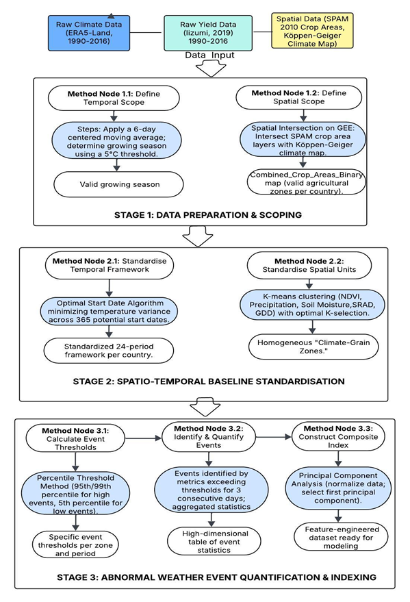
4.2.1 Stage 1: Data Preparation & Scoping
1. Defining Temporal Scope: Determining the Valid Growing Season To ensure the following steps of constructing homogeneous spatial units are efficient and effective (using a valid time range for weather variables), this research adopts a widely accepted methodology to define the growing season: a daily average temperature above or below a threshold (5°C) for more than six consecutive days (Nolan & Flanagan, 2020). We apply a two-step methodology:
The first step involves using a 6-day centred moving average to smooth the daily temperature dataset, extracting the first date point of six consecutive days exceeding 5°C, and the last date point of moving below 5°C.
The second step is to define the start and end months based on the calculated dates. For example, if the start date is after April 27, then the start month will be rounded up to May. This procedure ensures the use of K-means clustering for the climate-grain zones, utilising weather variables that precisely match the corresponding agricultural practices.
2. Defining Spatial Scope: Identifying Valid Agricultural Zones This procedure was completed on the Google Earth Engine platform, utilising two widely used and accepted datasets: Köppen-Geiger Climate Classification and SPAM 2010 V2r0. The former is a climate classification map that divides the global regions into different climate pattern zones, and the latter is used to get global agricultural production spatial distribution data.
We upload the SPAM 2010 dataset (production information map) and the Köppen-Geiger climate map to the GEE platform, then conduct a spatial intersection between these two maps to create a Combined_Crop_Areas_Binary map for each country, covering four crops. This method efficiently excludes regions and fields not used for agricultural purposes, obtaining a basic divided climate region that serves as a basis for the next step in building a set of climate-grain zones.
4.2.2 Stage 2: Spatial-Temporal Baseline Standardisation
1. Temporal Standardisation: Creating a Data-Driven 24-Period Framework The core of this methodology is to determine a start date for the 24-period division based on a date with the most balanced climate pattern for this 24-period period. For this procedure, we focused on the pre-selected country list and the EU as a whole region, given the relatively minor geographical area of each EU country.
- For each country, this algorithm loops through each date (a total of 365 dates) of the whole year, setting every day as a potential start date.
- For every potential start date, the algorithm calculates 24 consecutive 15-day periods for the year and obtains a vector containing the average temperatures for each period.
- Then this algorithm calculates the variance of this vector; this variance is used as the objective function, the smaller the variance, the more balanced the 24-period temperature distribution.
- The start date that yields the most minor variance is selected as the candidate start date for the country.
- Once the optimal annual division is identified, it produces a sequence of 24 consecutive periods, each with its own start date. From these 24 start dates, the one that falls in January and is the earliest in the calendar is selected as the final start date for that country.
These steps establish a standardised temporal framework for the following calculation, ensuring all countries have comparable 24×15-day periods as analysis units. Using this period-division method can better capture the change in weather patterns throughout the agricultural production timeline, avoiding excessive fluctuation in daily information or different seasonal patterns for each country, which would both introduce more noise into the model.
2. Spatial Standardisation: Constructing Homogeneous climate-grain zones This research applies the classic K-means clustering algorithm to divide the space data points into k distinct clusters, with each spatial zone exhibiting a high level of homogeneity. This ensures that the climate-grain zones reached from this method have a similar climate-weather pattern within the geographic border, which ensures scientific and less noisy model building.
In K-means clustering, the value of K is a crucial parameter that needs to be preset to determine the optimal K objectively, rather than being subjectively chosen. This research designed and implemented a systematic assessment framework and a chosen algorithm based on a well-accepted principle, to quantify the model performance with different K values. We employ a suite of three complementary evaluation metrics: the Silhouette Coefficient (a higher value indicates better performance), the Davies-Bouldin Index (DBI), which yields a lower value for a better model result, and the Calinski-Harabasz Index (CH), where a higher value is preferable. Based on the normalisation of these three metrics, we calculated a compound score.
The final choice of the best K is calculated by the three-layer algorithms below, which prioritise the quality and balance of the cluster:
1) Primary Path: The algorithm first filters the K value, which can result in the most balanced zones, with the most significant cluster proportion not exceeding 50%, on top of this, further selects the k with a well-structured cluster result, silhouette > 0.5, if multiple K meet this criteria, choose the value with highest silhouette, when silhouettes are the same, the composite score will make final decisions.
2) First Fallback Path: if for all the K which meet the balance criteria, but no one meets the 0.5 silhouette requirement, the best K will be selected by the highest silhouette, even if it is lower than 0.5, and the final choice is the same as determined by comparing the composite score.
3) Second Fallback Path: under specific situations, no K will meet the balance criteria; then the default choice will be the K with the highest composite score. This method ensures that, in every scenario, this algorithm will always return a robust K.
4.2.3 Stage 3: Abnormal Weather Event Quantification & Indexing
For effectively capturing the abnormal weather event, which is a key driving factor in building future models. This research designs a standard workflow from event identification to composite indices construction.
1. Calculating Event Thresholds This research employs the percentile threshold method as the primary identification standard, implemented on the Google Earth Engine (GEE) platform. Based on historical data covering 1990–2016 and dividing each year into precalculated 24×15-day periods, we calculate historical percentile per event and per period: high value events adopt 99th / 95th percentile (heatwave, 95th; extreme precipitation, flood runoff, storm wind speed, 99th); low value events utilizing 5th percentile threshold (cold wave, drought, and sunshine). This is the recommended method used in the IPCC AR6 WGI (2021) report, chapter 11 & chapter 12 (Seneviratne et al., 2021; Ranasinghe et al., 2021).
2. Identifying & Quantifying Events When the value for a specific weather statistic on a date exceeds the calculated threshold for three consecutive days (one day for the wind speed of a storm), we recognise it as one event and then store the statistical information for this event. Each geographic grid receives a unique value set (count for the number of repeated events, mean for the average value of this weather statistic, and max/min for the level of severity) for a specific period each year.
Then, the country-zone-level values (count of events, mean, maximum/minimum) were calculated by aggregating all the values from the geographic grids within the zone. As there will be many fragile areas within each zone, the final zone-level results will present as continuous values instead of discrete values, making them more suitable for building models. This method maintains the relative nature and spatio-temporal comparability of event definition.
3. Construction of the Composite Index Before implementing the PCA method to reduce the dimensions of the features, the table had 1613 rows (representing 13 countries with multiple zones spanning 27 years) and 508 columns (corresponding to seven categories of weather events, each with three statistics for 24 periods). To enhance the model’s performance and improve its interpretability, a unique statistic is calculated for each event, fully reflecting the impact of that event, by utilising the two-step PCA method, which integrates the three statistical values: count, mean, and min/max.
1) First step: We conduct normalisation and directional consistency (such as reversing the minimum value for cold wave, drought, and sunshine) to ensure the three statistics have the same directional impact on the final composite index and unify the scale of all input features.
2) Second step: The PCA method has been utilised to reduce dimension, and the first principal component was used as the composite index, which explains the most significant variance in the dataset. This method effectively decreases the complexity of the model and reduces multicollinearity among features.
When the three data processing stages are finished, the complex raw dataset of weather information has been transformed into a structured, information-intensive feature input for the first agricultural model building.
4.3 Part 2: Linking Physical to Financial
4.3.1 Rationale for Feature Selection: From Physical Impact to Financial Transmission
We choose a benchmark Wheat index in the financial market as the target variable for building the second time series model. However, we cannot directly use the abnormal events calculated in part 1 as input features, as the dataset’s scale is relatively small for robust model building, given that 24 periods of 27-year data only contain 648 data points. Moreover, the market fluctuates differently from agricultural production; daily data have a direct impact on the movement of market sentiment through information estimation and dissemination.
To accurately reflect the physical world, we do not choose weather factors randomly; we build our data selection methodology based on the core findings of the first model analysis. This methodology, based on the logic of the key influencer in agricultural production, will have a significant impact on both the supply and demand sides of the agricultural production market. Thus, financial market fluctuations should be based on the estimation of the futures market, especially the S&P GSCI wheat Index, which is calculated using production value-weighted futures contracts.
4.3.2 Feature Extraction and Engineering: Building the Time-Series Dataset
We utilise the standardised spatial unit, which is calculated in the previous steps (the climate-grain zones), to extract geographical gridded data for temperature and soil moisture and aggregate to zone level, thus we build a dataset for time series analysis, where each column represents a specific zone in each country’s weather data change over time. This dataset-building methodology establishes a precise link between the financial market and the physical world.
4.4 Conclusion
This chapter, through systematic data feature engineering, builds two standardised datasets: the highly homogeneous spatio-temporal units for the first agricultural model, and the logically internally linked dataset built using the most influential features from the first model as input variables for the second financial model.